Ruminations on a state championship
/If you grew up in Arkadelphia, you've likely heard stories about the state championships in which the Badger football team has played. In his Southern Fried Blog, Rex Nelson provides several accounts of the great Badger teams of the 1970s, which culminated in the 1979 state title. Most Arkadelphians know that team was coached by a first-year head coach, who was a young 25-year old named John Outlaw. Rex's profile on Coach Outlaw as part of a series of 2013 inductees into the Arkansas Sports Hall of Fame is a must read.

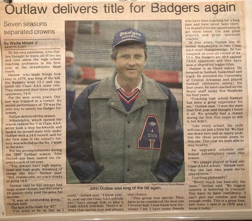
In 1987, Outlaw coached the Badgers to another state championship victory over White Hall.

The article below from the Siftings Herald memorialized the accomplishment:
A special thanks goes out to Chris Webb for posting these old news clippings on social media. I remember “Coach Webb” being the coach you wanted to run through a brick wall for in 7th grade football.
While I was at the ‘87 state title game, I was also only a five-year old little boy trying to stay warm, and don't remember it. The '87 Badgers were the first of any Arkansas high school football team to be nationally ranked in the USA Today Super 25 as seen below.


The ‘87 Badgers were also the first team in a lower classification to be ranked #1 overall in the state.
With a 51-26 win over Pea Ridge last Friday night, Arkadelphia will face Warren for the 4A state championship tomorrow. Who knew it would be 30 years before the Badgers would reach another state title game? Social media has been erupting all week with Arkadelphia High School graduates posting their favorite Badger memories, which motivated me to search around my house, as well as Don and Terri's, for footage of the '87 state title game. I found it on an old VHS tape in the last place I looked, tucked away in an old storage container long forgotten.
Coach Outlaw left for coaching opportunities in Texas after the '87 season. He was the Badgers' coach for 9 seasons, finishing with a record of 84-20-1. His final coaching record was 303-87-3. When he passed in December of 2011, Rex penned a fitting tribute about his life, which was about so much more than just football. A documentary about Coach Outlaw first premiered at the 2015 Hot Springs Documentary Film Festival. A few months after Coach Outlaw passed, so too did his top assistant and Clark County legend, Willie Tate. Again, Rex provided a fitting tribute to Coach Tate as he did with Coach Outlaw. As the Badgers are headed back to War Memorial Stadium tomorrow, our community is reminded of the last time we were there and the two men who were largely responsible for having the Badgers in the same position all those years ago.
After Coach Outlaw left for Texas, the Badgers finished 7-3 in '88, and missed the playoffs. A 1-9 season followed in '89. The next Badger team to have much success was the 1995 squad, who won a conference championship, but lost 3-2 in a first round home playoff game. In 1998, Arkadelphia hired its last state championship quarterback (featured in the '87 championship game video above), John Launius, to be head coach.

'98 was my sophomore year, and I had chosen not to play. As I watched friends and classmates improve to an overall 4-6 record, I knew I would be on the field with them in 1999. The most fun I had in high school was being a scout team tight end during the '99 season. I would be a backup my senior year to an all-state tight end who was a junior in 2000. Our '99 "psycho circus" defense featured two all-state linebackers that I had to face everyday in practice. The challenge was fun, and I enjoyed being part of a group that made our defense better.
One of the things Coach Launius instilled in us was taking advantage of opportunities. I can still hear him saying while addressing the team, "all you can ask for is a great opportunity!" He also preached accountability ("Be accountable, be a man, be a Badger!"). Our mantra the entire year was "11/12/99," which was the date of the first week of the state playoffs. At the end of the season, we beat Malvern to qualify as a 3 seed in an odd tie-breaker situation. We had given ourselves the opportunity Coach Launius preached about since his arrival as the Badger head coach. We drew Searcy in the first round, who had gone 8-2 that season. During the week before the game, Searcy sent us collector cups for the entire team from the "Searcy Senior Lions." Down 21-7 in the 3rd quarter, we rallied and sent the game to overtime at 21 apiece. We got the ball first in overtime, scored a touchdown on the first play, and held Searcy on four straight plays out of the end zone to win the first playoff game since the '87 state title team. Our starting center sent Searcy their collector cups back the following week.
Terri managed to catch some highlights.


The Wynne team we faced the next week had beaten us 28-7 in '98 in the regular season. Their '99 team featured Arrion Dixon, who would later play as a Razorback, and in the NFL. Their starting running back, Antonio Warren, would later play at Arkansas State. They also had a sophomore running back by the name of DeAngelo Williams, who at Memphis would become one of six collegiate players ever to rush for over 6,000 yards (three of these six won Heisman trophies), and just recently retired after a long NFL career. We lost the game 21-7.

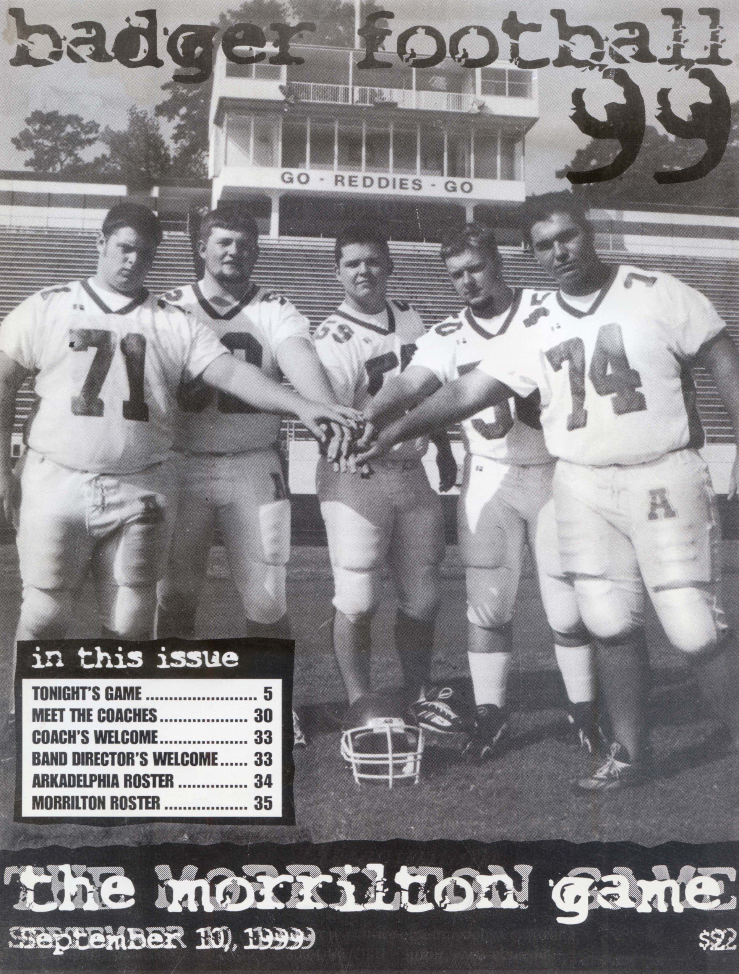
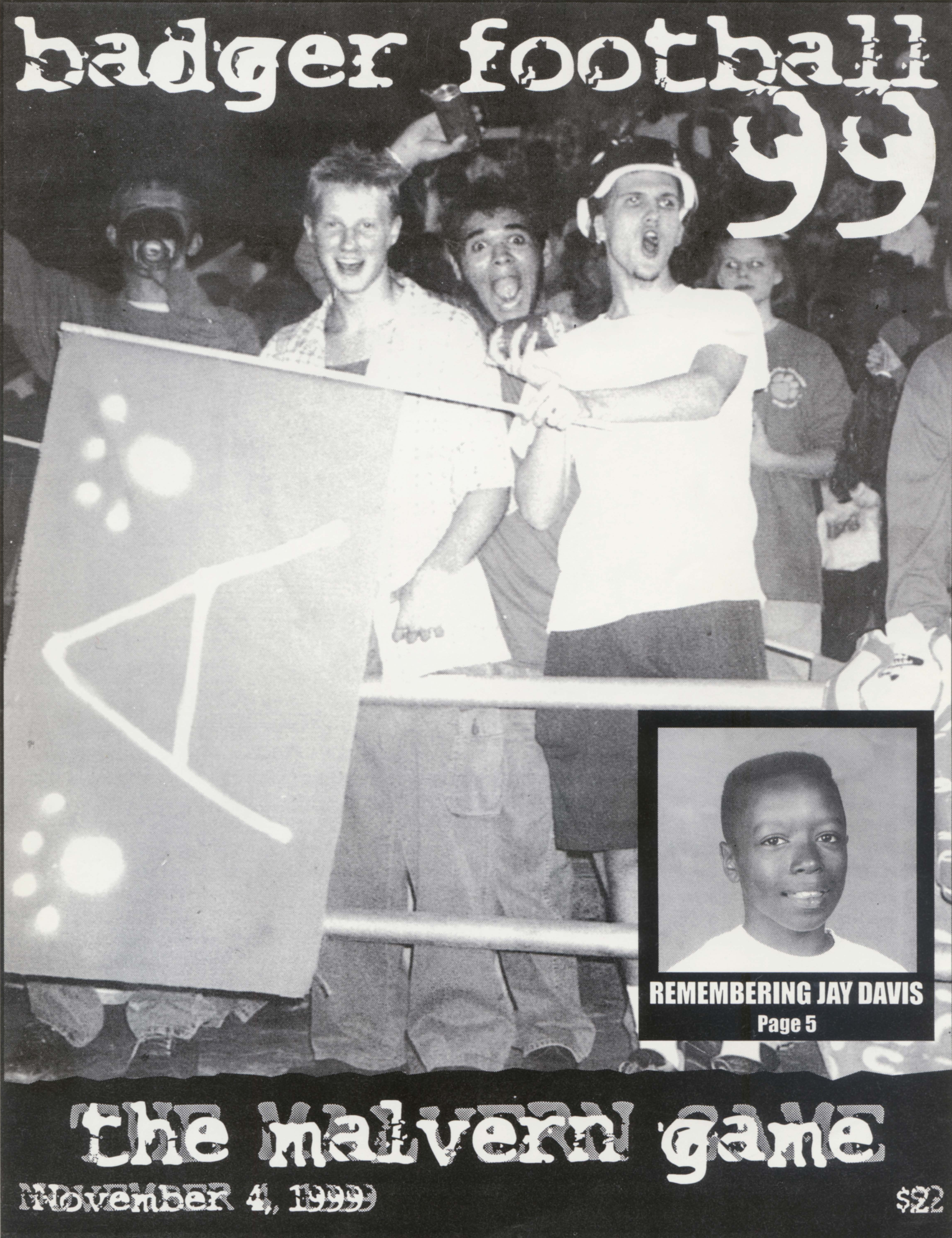
1999 Badger Football
There was much anticipation for the 2000 season. We knew we were going to be good, but the question everyone wondered, was how good? I think Coach Launius knew that too, and drilled a "one game at a time" approach into us.

2000 Badger Football
We knew we had a chance at a special year after beating Benton for the first time since '87. Benton was in a higher classification than us. Two weeks later we played Little Rock-Parkview, who was also in a higher classification.

A 40-7 beat down over Parkview gave us a lot of confidence. Perhaps we were too confident. We faced the undefeated Hope Bobcats the next week, whom we had beaten in Hope the previous season.

Hope won 21-7 that night in a tough, physical game. We finished the regular season 9-1, and earned a home playoff game against Newport.

Our strong safety had been hurt the week before against Malvern, which proved to be a costly injury. We couldn't stop the Greyhounds from running the ball. After our season ended at 9-2, I put together the team's highlight film, which started a hobby of digital video editing that I still have today. Below is part of the highlight film I put together:
Like Coach Outlaw, Coach Launius left for Texas a few years after I graduated in 2001. The Badgers didn't have much playoff success until J.R. Eldridge became the head coach for the 2011 season. Two years later he had the Badgers in the quarterfinals, where they lost by a touchdown at Warren. I knew back then Coach Eldridge would be playing for a championship eventually. That is borne out by the '17 team being among the top teams in both scoring offense, and scoring defense in the 4A classification.

Badger football is something that has always brought the Arkadelphia community together. It did before my time, during my time, and is currently doing so now. It's been a fun week to live here. Reading old articles from teams in the past, seeing old pictures from the Outlaw days, and seeing my high school coach quarterback our last state title team has made me realize that while the '17 team is standing on all of our collective shoulders, we're all going to be standing on theirs tomorrow.